By Jack DiBari

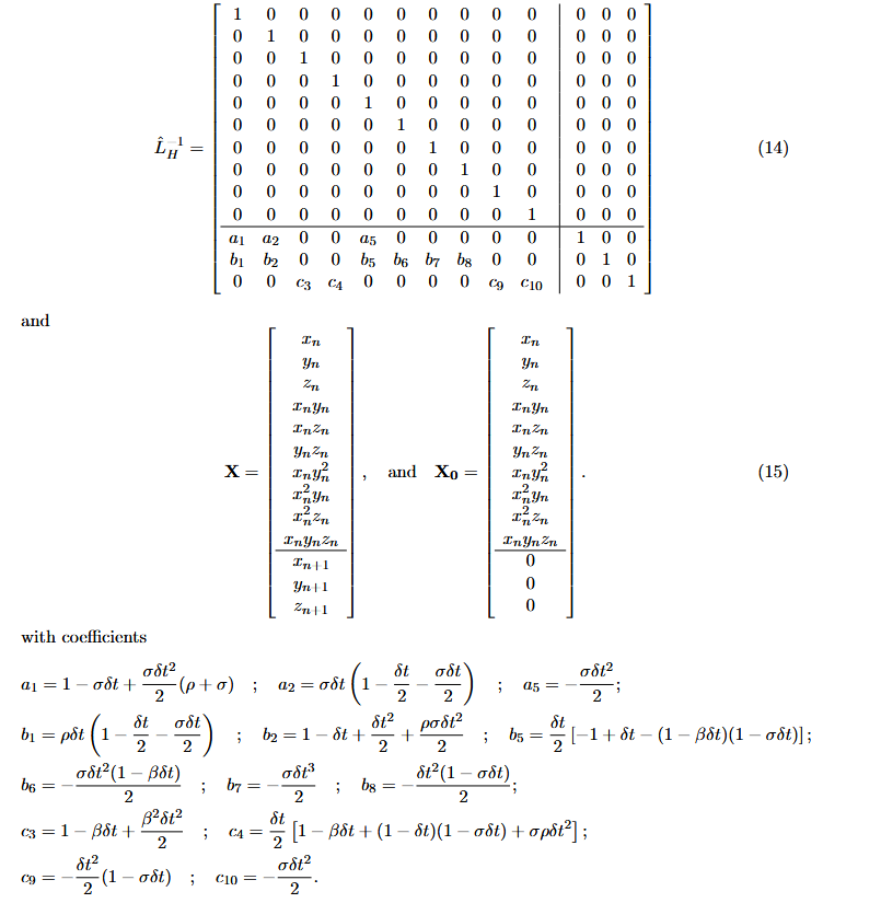
A scheme is created to implement the Lorenz Attractor. The inverse Heun-matrix of which is shown below:

Previous work

Quantum Presentation

In Python, this can be simply implemented by multiplying the matrix with the initial values(matrix multiplication):

@qml.qnode(dev)
def apply_operation_default_qubit(op, x_0):
    qml.AmplitudeEmbedding(x_0, wires=range(num_qubits), normalize=False)
    qml.QubitUnitary(op, wires=range(num_qubits))
    return qml.probs(wires=range(num_qubits))

Implementing the quantum simulator

First, we create a device, specifying the back-end used and the wires.

dev = qml.device('default.qubit', wires=num_qubits)

devices used

Apart from the default device, we have several devices options, as listed here. Each of these is a backend for executing quantum circuits, and have their own advantages and disadvantages. Our ‘default.qubit’ is good for general-purpose operations on small-to-medium sized circuits and prototyping, and it uses a statevector representation. Several other devices will be considered in this simulation.

‘default.mixed’: a mixed-state simulator of qubit-based quantum circuit architectures. It is more memory and compute-intensive than our ‘default.qubit’, and it is able to simulate open quantum systems, decoherence, and noise. ‘lightning.qubit’: a more performant state simulator of qubit-based quantum circuit architectures written in C++. JAX backend: Uses a JAX backend. JAX is a Python library for high-performance numerical computation.

number of qubits

The inverse-Heun matrix contains 13 rows and 13 columns. This will be block-encoded to make it 32 rows and 32 columns, which requires 5 qubits overall.

The quantum circuit

In Pennylane, a quantum circuit or function is contained in a “QNode,” which is simply a Python function with a decorator. Our QNode will embed X0 into the amplitude vector, apply the unitary matrix, and then return the probability amplitudes.

@qml.qnode(dev)
def apply_operation_default_qubit(op, x_0):
    qml.AmplitudeEmbedding(x_0, wires=range(num_qubits), normalize=False)
    qml.QubitUnitary(op, wires=range(num_qubits))
    return qml.probs(wires=range(num_qubits))

making it unitary

Using Pennylane’s BlockEncode function, the inverse Heun matrix can be block-encoded:

op = qml.BlockEncode(inverse_heun, wires=range(num_qubits))

The BlockEncode function, which is described here, encodes a matrix in the top-left block of a 2×2 matrix, shown here:

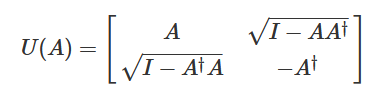
If the norm of A is greater than one, it is normalized to make sure that the resulting U(A) is unitary. The value that is used to normalize this (the normalization constant) is stored in a special variable which we will retrieve later. In our case, many parameters cause the norm of A to be greater than one, so it will be important for us to have this constant, which we will have to multiply with the output of the system to get a de-normalized result.

preparing the initial state

The initial state is created by putting initial values in an array, normalizing the values, and using AmplitudeEmbedding to populate the initial state. The values must be normalized, or AmplitudeEmbedding won’t work correctly.

X_01 = np.array([x,y,z,x*y,x*z,y*z,x*(y*y),(x*x)*y,(x*x)*z,x*y*z, 0, 0, 0], dtype=np.float64)
X_0[:len(X_01)] = X_01
norm = np.linalg.norm(output)
if norm != 0:
    output /= norm

applying the system

The quantum circuit can be applied by running apply_operation_default_qubit with the block-encoded inverse-Heun matrix and initial value array as parameters.

output = apply_operation_default_qubit(op.matrix(), output)

output of the system

Applying the quantum circuit should result in a complex-valued Numpy array of length 32 float64 elements. The first 13 elements represent the normalized X (from equation 15) and elements 11-13 represent the next x, y, and z value of the Lorenz system. By getting the real values, multiplying by the norm, and multiplying by the normalization constant if necessary, the next x, y, and z values can be retrieved.

result = output[10:13].real * norm
if alpha > 1:
    result *= alpha
x = result[0]
y = result[1]
z = result[2]

interpreting results

Using the following parameters, the system can be graphed, shown below. Plots of x vs. t, y vs. t, z vs. t, and x, y, and z were generated.

parameters:

h: 0.001, sigma: 10, rho: 28, beta: 8/3, initial_values: [0.1, 0.1, 0.1], alpha: 1, iterations: 255, g: 80

x vs. t:

{{CODE1}}

y vs. t:

{{CODE2}}

z vs. t:

{{CODE3}}

graph of x, y, and z:

{{CODE5}}

timing comparison:

{{CODE4}}

improvements

error due to normalization

In theory, having to recalculate and re-normalize the initial value array every iteration is unnecessary and takes extra time. As the initial value array is normalized, and the probability output amplitudes are normalized, the output should be able to be fed back into the input every iteration. qml.probs() always returns the probabilities of measuring each state, as the magnitude of the amplitude of each, squared. After each iteration, the square root of the output can be calculated, and the x, y, and z values saved. Then after all the iterations the alpha can be multiplied and the output scaled.

sparse matrix

Around 60% of the elements in op are zeros, which means that some of the methods designed for sparse matrices could be applied. However, support of sparse matrix operations within Pennylane is not fully supported.

negative probability amplitudes

In Pennylane, qml.state() returns the full quantum statevector of the circuit. It is complex-valued, and includes phase information. It exists only on simulators, and not on hardware devices or shot-based devices. On the other hand, qml.probs() returns the probability distribution of measuring the basis states. This measurement does not preserve complex values or phase information. Because of this, the sign of the output values will have to be estimated. Different measurements other than probabilities can be used to reveal sign. A link to the full writeup can be found here: https://docs.google.com/document/d/17vp9FzwQVsBenv7VAOJEFmcwENyco8bR2WMxlWixNS4/edit?usp=sharing

Welcome to Old Dominion University – WordPress. This is your first post. Edit or delete it, then start blogging!